Evaluate the performance of a fitted pipeline
factory_model_performance_r.RdPerformance metrics on the test set.
factory_model_performance_r(pipe, x_train, y_train, x_test, y_test, metric)
Arguments
| x_train | Data frame. Training data (predictor). |
|---|---|
| y_train | Vector. Training data (response). |
| x_test | Data frame. Test data (predictor). |
| y_test | Vector. Test data (response). |
| metric | String. Scorer that was used in pipeline tuning ("accuracy_score", "balanced_accuracy_score", "matthews_corrcoef", "class_balance_accuracy_score") |
Value
A list of length 5:
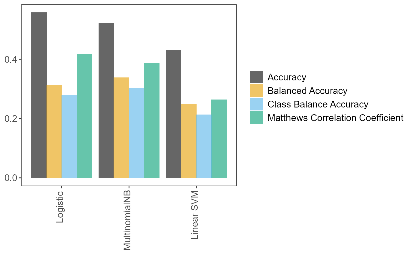
pipeThe fittedScikit-learn/imblearnpipeline.tuning_resultsData frame. All (hyper)parameter values and models tried during fitting.predVector. The predictions on the test set.accuracy_per_classData frame. Accuracies per class.p_compare_models_barA bar plot comparing the mean scores (of the user-suppliedmetricparameter) from the cross-validation on the training set, for the best (hyper)parameter values for each learner.
Note
Returned object tuning_results lists all (hyper)parameter values
tried during pipeline fitting, along with performance metrics. It is
generated from the Scikit-learn output that follows pipeline fitting.
It is derived from attribute cv_results_
with some modifications. In R, cv_results_ can be accessed following
fitting of a pipeline with pxtextmineR::factory_pipeline_r or by
calling function pxtextmineR::factory_model_performance_r. Say that
the fitted pipeline is assigned to an object called pipe, and that the
pipeline performance is assigned to an object called pipe_performance.
Then, cv_results_ can be accessed with pipe$cv_results_ or
pipe_performance$cv_results_.
NOTE: After calculating performance metrics on the test set,
pxtextmineR::factory_model_performance_r fits the pipeline on the
whole dataset (train + test). Hence, do not be surprised that the
pipeline's score() method will now return a dramatically improved score
on the test set- the refitted pipeline has now "seen" the test dataset
(see Examples). The re-fitted pipeline will perform much better on fresh
data than the pipeline fitted on x_train and y_train only.
References
Pedregosa F., Varoquaux G., Gramfort A., Michel V., Thirion B., Grisel O., Blondel M., Prettenhofer P., Weiss R., Dubourg V., Vanderplas J., Passos A., Cournapeau D., Brucher M., Perrot M. & Duchesnay E. (2011), Scikit-learn: Machine Learning in Python. Journal of Machine Learning Research 12:2825–-2830.
Examples
# Prepare training and test sets data_splits <- pxtextmineR::factory_data_load_and_split_r( filename = pxtextmineR::text_data, target = "label", predictor = "feedback", test_size = 0.90) # Make a small training set for a faster run in this example # Let's take a look at the returned list str(data_splits)#> List of 6 #> $ x_train :'data.frame': 1033 obs. of 1 variable: #> ..$ predictor: chr [1:1033] "Very helpful and friendly." "Prompt appointment - information delivered clearly video appointment but everything worked well. Tian was very kind. " "FIrst Class" "Be a bit quicker when they are discharging you." ... #> ..- attr(*, "pandas.index")=Int64Index([5503, 2371, 3214, 8067, 5880, 5011, 9713, 5085, 1416, 3565, #> ... #> 1879, 3833, 5913, 130, 7556, 1177, 1287, 2813, 8771, 1690], #> dtype='int64', length=1033) #> $ x_test :'data.frame': 9301 obs. of 1 variable: #> ..$ predictor: chr [1:9301] "Absolutely happy wIth everythIng, very nIce people." "More staff At times the ward felt understaffed and with such poorly children" "Always lIstened to regardIng any Issues." "Listen. \nStaff communication with each other was excellent, it gave me a much better experience this time. T"| __truncated__ ... #> ..- attr(*, "pandas.index")=Int64Index([ 2663, 8720, 2772, 1634, 7900, 1815, 2534, 1766, 10026, #> 7140, #> ... #> 1213, 5090, 1385, 5740, 4183, 7520, 2770, 2408, 5436, #> 1266], #> dtype='int64', length=9301) #> $ y_train : chr [1:1033(1d)] "Care received" "Access" "Care received" "Transition/coordination" ... #> ..- attr(*, "dimnames")=List of 1 #> .. ..$ : chr [1:1033] "5503" "2371" "3214" "8067" ... #> $ y_test : chr [1:9301(1d)] "Care received" "Staff" "Communication" "Communication" ... #> ..- attr(*, "dimnames")=List of 1 #> .. ..$ : chr [1:9301] "2663" "8720" "2772" "1634" ... #> $ index_training_data: int [1:1033] 5503 2371 3214 8067 5880 5011 9713 5085 1416 3565 ... #> $ index_test_data : int [1:9301] 2663 8720 2772 1634 7900 1815 2534 1766 10026 7140 ...# Fit the pipeline pipe <- pxtextmineR::factory_pipeline_r( x = data_splits$x_train, y = data_splits$y_train, tknz = "spacy", ordinal = FALSE, metric = "accuracy_score", cv = 2, n_iter = 10, n_jobs = 1, verbose = 3, learners = c("SGDClassifier", "MultinomialNB") ) # (SGDClassifier represents both logistic regression and linear SVM. This # depends on the value of the "loss" hyperparameter, which can be "log" or # "hinge". This is set internally in factory_pipeline_r). # Assess model performance pipe_performance <- pxtextmineR::factory_model_performance_r( pipe = pipe, x_train = data_splits$x_train, y_train = data_splits$y_train, x_test = data_splits$x_test, y_test = data_splits$y_test, metric = "accuracy_score") names(pipe_performance)#> [1] "pipe" "tuning_results" "pred" #> [4] "accuracy_per_class" "p_compare_models_bar"# Let's compare pipeline performance for different tunings with a range of # metrics averaging the cross-validation metrics for each fold. pipe_performance$ tuning_results %>% dplyr::select(learner, dplyr::contains("mean_test"))#> learner mean_test_Accuracy mean_test_Balanced Accuracy #> 2 Logistic 0.5575941 0.3137440 #> 0 Logistic 0.5324266 0.3695176 #> 6 MultinomialNB 0.5217639 0.3385196 #> 5 Logistic 0.5169227 0.3449101 #> 4 MultinomialNB 0.4375384 0.3138912 #> 3 Linear SVM 0.4307424 0.2475875 #> 1 Logistic 0.4288344 0.2762078 #> 7 Linear SVM 0.3988275 0.2486355 #> 8 MultinomialNB 0.3987862 0.2584215 #> 9 MultinomialNB 0.3678272 0.2691415 #> mean_test_Matthews Correlation Coefficient mean_test_Class Balance Accuracy #> 2 0.4173449 0.2784928 #> 0 0.4026087 0.3276369 #> 6 0.3868081 0.3025500 #> 5 0.3850773 0.3081798 #> 4 0.3069311 0.2523217 #> 3 0.2640922 0.2134373 #> 1 0.2682233 0.2329601 #> 7 0.2369170 0.2099112 #> 8 0.2538160 0.2117422 #> 9 0.2251304 0.1871887# A glance at the (hyper)parameters and their tuned values pipe_performance$ tuning_results %>% dplyr::select(learner, dplyr::contains("param_")) %>% str()#> 'data.frame': 10 obs. of 22 variables: #> $ learner : chr "Logistic" "Logistic" "MultinomialNB" "Logistic" ... #> $ param_sampling__kw_args : chr "{'up_balancing_counts': 800}" "{'up_balancing_counts': 300}" "{'up_balancing_counts': 800}" "{'up_balancing_counts': 800}" ... #> $ param_preprocessor__texttr__text__transformer__use_idf :List of 10 #> ..$ : logi FALSE #> ..$ : logi TRUE #> ..$ : logi TRUE #> ..$ : logi FALSE #> ..$ : logi FALSE #> ..$ : logi FALSE #> ..$ : logi FALSE #> ..$ : logi TRUE #> ..$ : logi TRUE #> ..$ : logi TRUE #> $ param_preprocessor__texttr__text__transformer__tokenizer : chr "<pxtextmining.helpers.tokenization.LemmaTokenizer object at 0x000000006F3FA730>" "<pxtextmining.helpers.tokenization.LemmaTokenizer object at 0x000000006F3FA730>" "<pxtextmining.helpers.tokenization.LemmaTokenizer object at 0x000000006F3FAC10>" "<pxtextmining.helpers.tokenization.LemmaTokenizer object at 0x000000006F3FA730>" ... #> $ param_preprocessor__texttr__text__transformer__preprocessor: chr "<function text_preprocessor at 0x00000000665D93A0>" "<function text_preprocessor at 0x00000000665D93A0>" "<function text_preprocessor at 0x00000000665D93A0>" "<function text_preprocessor at 0x00000000665D93A0>" ... #> $ param_preprocessor__texttr__text__transformer__norm :List of 10 #> ..$ : NULL #> ..$ : chr "l2" #> ..$ : chr "l2" #> ..$ : chr "l2" #> ..$ : NULL #> ..$ : chr "l2" #> ..$ : chr "l2" #> ..$ : chr "l2" #> ..$ : chr "l2" #> ..$ : chr "l2" #> $ param_preprocessor__texttr__text__transformer__ngram_range : chr "(1, 3)" "(1, 3)" "(1, 3)" "(1, 3)" ... #> $ param_preprocessor__texttr__text__transformer__min_df :List of 10 #> ..$ : int 1 #> ..$ : int 1 #> ..$ : int 1 #> ..$ : int 1 #> ..$ : int 1 #> ..$ : int 1 #> ..$ : int 3 #> ..$ : int 3 #> ..$ : int 3 #> ..$ : int 3 #> $ param_preprocessor__texttr__text__transformer__max_df :List of 10 #> ..$ : num 0.7 #> ..$ : num 0.7 #> ..$ : num 0.95 #> ..$ : num 0.95 #> ..$ : num 0.95 #> ..$ : num 0.7 #> ..$ : num 0.7 #> ..$ : num 0.95 #> ..$ : num 0.7 #> ..$ : num 0.7 #> $ param_preprocessor__texttr__text__transformer : chr "TfidfVectorizer(max_df=0.7, ngram_range=(1, 3), norm=None,\n preprocessor=<function text_preproc"| __truncated__ "TfidfVectorizer(max_df=0.7, ngram_range=(1, 3), norm=None,\n preprocessor=<function text_preproc"| __truncated__ "TfidfVectorizer()" "TfidfVectorizer(max_df=0.7, ngram_range=(1, 3), norm=None,\n preprocessor=<function text_preproc"| __truncated__ ... #> $ param_preprocessor__sentimenttr__scaler__scaler__n_bins :List of 10 #> ..$ : int 8 #> ..$ : int 4 #> ..$ : int 8 #> ..$ : int 8 #> ..$ : int 4 #> ..$ : int 4 #> ..$ : int 8 #> ..$ : int 8 #> ..$ : int 8 #> ..$ : int 4 #> $ param_preprocessor__sentimenttr__scaler__scaler : chr "KBinsDiscretizer(n_bins=8, strategy='kmeans')" "KBinsDiscretizer(n_bins=8, strategy='kmeans')" "KBinsDiscretizer(strategy='kmeans')" "KBinsDiscretizer(n_bins=8, strategy='kmeans')" ... #> $ param_preprocessor__lengthtr__scaler__scaler : chr "KBinsDiscretizer(n_bins=3, strategy='kmeans')" "KBinsDiscretizer(n_bins=3, strategy='kmeans')" "KBinsDiscretizer(n_bins=3, strategy='kmeans')" "KBinsDiscretizer(n_bins=3, strategy='kmeans')" ... #> $ param_featsel__selector__score_func : chr "<function chi2 at 0x00000000665C14C0>" "<function chi2 at 0x00000000665C14C0>" "<function chi2 at 0x00000000665C14C0>" "<function chi2 at 0x00000000665C14C0>" ... #> $ param_featsel__selector__percentile :List of 10 #> ..$ : int 70 #> ..$ : int 100 #> ..$ : int 85 #> ..$ : int 70 #> ..$ : int 70 #> ..$ : int 100 #> ..$ : int 85 #> ..$ : int 100 #> ..$ : int 70 #> ..$ : int 85 #> $ param_featsel__selector : chr "SelectPercentile(percentile=70,\n score_func=<function chi2 at 0x00000000665C14C0>)" "SelectPercentile(percentile=70,\n score_func=<function chi2 at 0x00000000665C14C0>)" "SelectPercentile(percentile=70,\n score_func=<function chi2 at 0x00000000665C14C0>)" "SelectPercentile(percentile=70,\n score_func=<function chi2 at 0x00000000665C14C0>)" ... #> $ param_clf__estimator__penalty :List of 10 #> ..$ : chr "l2" #> ..$ : chr "elasticnet" #> ..$ : num NaN #> ..$ : chr "l2" #> ..$ : num NaN #> ..$ : chr "elasticnet" #> ..$ : chr "l2" #> ..$ : chr "l2" #> ..$ : num NaN #> ..$ : num NaN #> $ param_clf__estimator__max_iter :List of 10 #> ..$ : int 10000 #> ..$ : int 10000 #> ..$ : num NaN #> ..$ : int 10000 #> ..$ : num NaN #> ..$ : int 10000 #> ..$ : int 10000 #> ..$ : int 10000 #> ..$ : num NaN #> ..$ : num NaN #> $ param_clf__estimator__loss :List of 10 #> ..$ : chr "log" #> ..$ : chr "log" #> ..$ : num NaN #> ..$ : chr "log" #> ..$ : num NaN #> ..$ : chr "hinge" #> ..$ : chr "log" #> ..$ : chr "hinge" #> ..$ : num NaN #> ..$ : num NaN #> $ param_clf__estimator__class_weight : chr "None" "None" "nan" "None" ... #> $ param_clf__estimator : chr "SGDClassifier(loss='log', max_iter=10000)" "SGDClassifier(loss='log', max_iter=10000)" "MultinomialNB()" "SGDClassifier(loss='log', max_iter=10000)" ... #> $ param_clf__estimator__alpha :List of 10 #> ..$ : num NaN #> ..$ : num NaN #> ..$ : num 0.1 #> ..$ : num NaN #> ..$ : int 1 #> ..$ : num NaN #> ..$ : num NaN #> ..$ : num NaN #> ..$ : int 1 #> ..$ : int 1 #> - attr(*, "pandas.index")=Int64Index([2, 0, 6, 5, 4, 3, 1, 7, 8, 9], dtype='int64')# Accuracy per class pipe_performance$accuracy_per_class#> class counts accuracy #> 1 Access 370 0.08648649 #> 2 Care received 3027 0.78328378 #> 3 Communication 786 0.27480916 #> 4 Couldn't be improved 1533 0.89954338 #> 5 Dignity 128 0.03906250 #> 6 Environment/ facilities 449 0.26057906 #> 7 Miscellaneous 318 0.48427673 #> 8 Staff 2560 0.59140625 #> 9 Transition/coordination 130 0.08461538# Learner performance barplot pipe_performance$p_compare_models_bar# Remember that we tried three models: Logistic regression (SGDClassifier with # "log" loss), linear SVM (SGDClassifier with "hinge" loss) and MultinomialNB. # Do not be surprised if one of these models does not show on the plot. # There are numerous values for the different (hyper)parameters (recall, # most of which are set internally) and only `n_iter = 10` iterations in this # example. As with `factory_pipeline` the choice of which (hyper)parameter # values to try out is random, one or more classifiers may not be chosen. # Increasing `n_iter` to a larger number would avoid this, at the expense of # longer fitting times (but with a possibly more accurate pipeline). # Predictions on test set preds <- pipe_performance$pred head(preds)#> [1] "Care received" "Care received" #> [3] "Care received" "Staff" #> [5] "Environment/ facilities" "Care received"################################################################################ # NOTE!!! # ################################################################################ # After calculating performance metrics on the test set, # pxtextmineR::factory_model_performance_r fits the pipeline on the WHOLE # dataset (train + test). Hence, do not be surprised that the pipeline's # score() method will now return a dramatically improved score on the test # set- the refitted pipeline has now "seen" the test dataset. pipe_performance$pipe$score(data_splits$x_test, data_splits$y_test)#> [1] 0.9823675pipe$score(data_splits$x_test, data_splits$y_test)#> [1] 0.9823675# We can confirm this score by having the re-fitted pipeline predict x_test # again. The predictions will be better and the new accuracy score will be # the inflated one. preds_refitted <- pipe$predict(data_splits$x_test) score_refitted <- data_splits$y_test %>% data.frame() %>% dplyr::rename(true = '.') %>% dplyr::mutate( pred = preds_refitted, check = true == preds_refitted, check = sum(check) / nrow(.) ) %>% dplyr::pull(check) %>% unique() score_refitted#> [1] 0.9823675# Compare this to the ACTUAL performance on the test dataset preds_actual <- pipe_performance$pred score_actual <- data_splits$y_test %>% data.frame() %>% dplyr::rename(true = '.') %>% dplyr::mutate( pred = preds_actual, check = true == preds_actual, check = sum(check) / nrow(.) ) %>% dplyr::pull(check) %>% unique() score_actual#> [1] 0.6234813score_refitted - score_actual#> [1] 0.3588861